A LMM or GLMM alternative to ratio paired t-test is the best practice to plot the model
Data From Fig 3b – The TAS1R2 G-protein-coupled receptor is an ambient glucose sensor in skeletal muscle that regulates NAD homeostasis and mitochondrial capacity
The researchers analyzed figure 3b with a ratio paired t-test, which is a special case of a linear mixed model with a log-transformed response. A generalized linear mixed model with a Gamma distribution and log link is an alternative. An advantage to fitting the LMM or GLMM is asymmetric confidence intervals of the group means that reflect the skew of the data. Plot the model!
linear mixed model
ratio paired t-test
generalized linear mixed model
ggplot
Author
Jeff Walker
Published
June 8, 2024
Modified
October 2, 2024
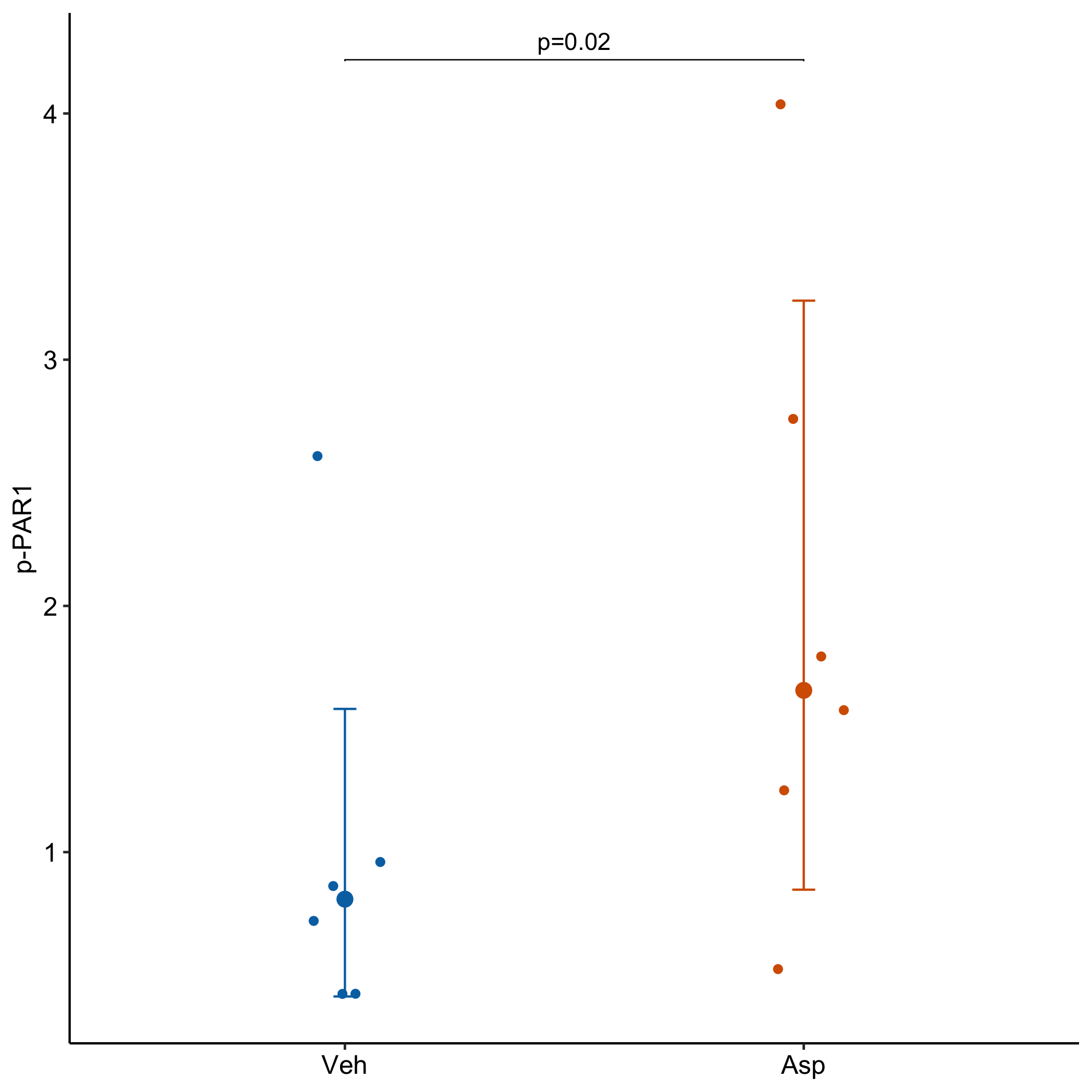
ggplot better-than-replication of Fig 3b from the article. It’s better than because the confidence intervals from the model are asymmetric and reflect the right (upward) skew of the data
The researchers engineered mice to express human TAS1R2 receptor in the muscles of muscle-specific TAS1R2 knockout (mKO) mice. Aspartame is a TAS1R2 agonist in humans but not mice. Presumably Saline was injected in muscle on one side and Aspartame on the other side of the same mouse, so mouse is a block, hence the ratio paierd t-test.
Treatments
Veh – Saline? injected into mTg mice muscle
Asp – Aspartame injected into mTg mice muscle
Setup
Import and Wrangle
Code
data_from <-"The TAS1R2 G-protein-coupled receptor is an ambient glucose sensor in skeletal muscle that regulates NAD homeostasis and mitochondrial capacity"file_name <-"41467_2024_49100_MOESM5_ESM.xlsx"file_path <-here(data_folder, data_from, file_name)fig3b_wide <-read_excel(file_path,sheet ="Fig.3b",range ="B7:C13",col_names =TRUE) |>data.table()setnames(fig3b_wide, old =names(fig3b_wide), new =c("Veh", "Asp"))fig3b_wide[, mouse :=paste0("mouse_", .I)]fig3b <-melt(fig3b_wide,id.vars ="mouse",variable.name ="genotype",value.name ="ppar1")# output as clean excel filefileout_name <-"fig3b-RCBD-The TAS1R2 G-protein-coupled receptor is an ambient glucose sensor in skeletal muscle that regulates NAD homeostasis and mitochondrial capacity.xlsx"fileout_path <-here(data_folder, data_from, fileout_name)write_xlsx(fig3b, fileout_path)
Fit the model
The paired t-test is a special case of a linear mixed model – specifically a linear mixed model with a single fixed factor and a single random intercept. For the ratio paired t-test, simply fit the model to the log transformed response.
For this experiment, genotype is the fixed factor, and mouse is the block, so will be fit as a random factor. Note that I include the log transorm in the model formula, which signals the emmeans package to report the results on the response scale, which makes the treatment effect a ratio instead of a log ratio.
 contrast  ratio    SE df lower.CL upper.CL null t.ratio p.value
 Asp / Veh  2.05 0.434  5     1.19     3.53    1   3.386  0.0195

Degrees-of-freedom method: kenward-roger
Confidence level used: 0.95
Intervals are back-transformed from the log scale
Tests are performed on the log scale
The treatment effect (“ratio”) is the geometric mean (not the mean!) of the ratios Asp/Veh. Ratios are nice for interpretation: p-PAR1 levels in the Aspartame treatment are 2.05 times the levels in the Vehicle treatment.
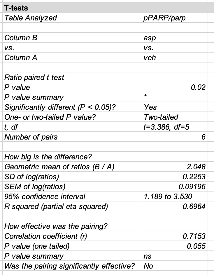
The effect (ratio of Asp/Veh), confidence interval, and p-value from the LMM are the same as in the archived table shown below.
Note the asymetric intervals! This is because the intevals were computed on the log-transformed values and then backtransformed to the scale of the response.
The ratio paired t-test is a one-sample t-test of the log of the Asp/Veh ratios. For a null hypothesis of no effect, we expect the geometric mean of the ratios to be 1, so the log of this to be 0.
Code
a <- fig3b[genotype =="Veh", ppar1]b <- fig3b[genotype =="Asp", ppar1]log_ba <-log(b/a)t.test(log_ba, mu =0)
    One Sample t-test

data:  log_ba
t = 3.3863, df = 5, p-value = 0.01954
alternative hypothesis: true mean is not equal to 0
95 percent confidence interval:
 0.1727216 1.2613696
sample estimates:
mean of x
0.7170456
These are the same values as the archived values and the results from the linear mixed model above.
The ratio paired t-test is just a paired t-test of the log-transformed response
This was implied above but here are the results to verify this.
    Paired t-test

data:  log_b and log_a
t = 3.3863, df = 5, p-value = 0.01954
alternative hypothesis: true mean difference is not equal to 0
95 percent confidence interval:
 0.1727216 1.2613696
sample estimates:
mean difference
      0.7170456
A generalized linear mixed model is a more modern way of analyzing these data
Intensity levels often have a non-Normal distribution that is characterized by a right skew and a variance that increases with the mean (you can see this even with the small sample in Fig 3b. A modern way to analyze data like this is a generalized linear model, or, since we have a RBCD, a generalized linear mixed model.
Here, I fit a GLMM using the Gamma distribution, which is useful for continuous, positive data.
 contrast  ratio    SE  df asymp.LCL asymp.UCL null z.ratio p.value
 Asp / Veh  2.05 0.398 Inf       1.4         3    1   3.715  0.0002

Confidence level used: 0.95
Intervals are back-transformed from the log scale
Tests are performed on the log scale
Huh. This is equivalent to the LMM/ratio paired t-test, except its an “asymptotic test”, so the p-value is optimistic and the confidence interval is narrow.
I was expecting the effect to be the ratio of the means and not geometric mean of the ratios. This would have been the case with a GLM without the random intercept – see below, but first, here are the different means (expand the code block to see what each is)
Code
a <- fig3b[genotype =="Veh", ppar1]b <- fig3b[genotype =="Asp", ppar1]mean(b)/mean(a) # ratio of means
[1] 1.99065
Code
exp(log(mean(b)) -log(mean(a))) # difference of log transformed means backtransformed =
[1] 1.99065
Code
exp(mean(log(b)) -mean(log(a))) # means of log transformed data backtransformed = geometric mean
[1] 2.048372
Code
prod(b/a)^(1/length(b/a)) # geometric mean computation 1
[1] 2.048372
Code
exp(mean(log(b/a))) # geometric mean computation 2
[1] 2.048372
And here is the GLM to show that the effect is the ratio of means
 contrast  ratio    SE  df asymp.LCL asymp.UCL null z.ratio p.value
 Asp / Veh  1.99 0.702 Inf     0.998      3.97    1   1.953  0.0508

Confidence level used: 0.95
Intervals are back-transformed from the log scale
Tests are performed on the log scale